
R Tutorials
SPARQL for R Tutorial - Linked Open Piracy
By Willem Robert van Hage. Acknowledgments to Jesper Hoeksema and Marieke van Erp.
This tutorial shows how to do a visual analysis and basic statistical analysis of the data in the Linked Open Piracy data set. It makes use of the SPARQL Package for R and the ggmap package.
The SPARQL Package allows you to directly import results of SPARQL SELECT queries into the statistical environment of R as a data frame. That means you can directly perform statistical analysis on data sets on the web. For example, you can use the following R code to get data from the Linked Open Piracy SPARQL end point described below. The complete script is available for download: sparql_lop.R.
Accessing the data
At first, make sure that you have recent versions of the two R packages SPARQL, ggmap, and mapproj installed. Load the packages by calling:library(SPARQL) library(ggmap)
Define the endpoint that will provide you with the triples by
endpoint <- "http://semanticweb.cs.vu.nl/lop/sparql/"
State that there are no further options to send to the SPARQL server. These options are sent as HTTP parameters and differ per end point. For example, Jena Fuseki can take the option "output=xml" to dictate that it should return XML, SWI-Prolog Cliopatria can take "entailment=rdfs" or "entailment=none" to state which kind of reasoning to apply.
options <- NULL
For a local Jena Fuseki installation hosting the same data in the LOP graph you can use the following options (uncommented, i.e., without the leading #):
# endpoint <- "http://localhost:3030/lop/query"
# options <- "output=xml"
To shorten the URIs of the data that we get back, use some namespace declarations like this
prefix <- c("lop","http://semanticweb.cs.vu.nl/poseidon/ns/instances/",
            "eez","http://semanticweb.cs.vu.nl/poseidon/ns/eez/")
sparql_prefix <- "PREFIX sem: <http://semanticweb.cs.vu.nl/2009/11/sem/>
                  PREFIX poseidon: <http://semanticweb.cs.vu.nl/poseidon/ns/instances/>
                  PREFIX eez: <http://semanticweb.cs.vu.nl/poseidon/ns/eez/>
                  PREFIX wgs84: <http://www.w3.org/2003/01/geo/wgs84_pos#>
                  PREFIX rdfs: <http://www.w3.org/2000/01/rdf-schema#>
"
The data you will now be able to access follows the Simple Event Model schema. An example of the structure of the graphs in the triple store is shown below.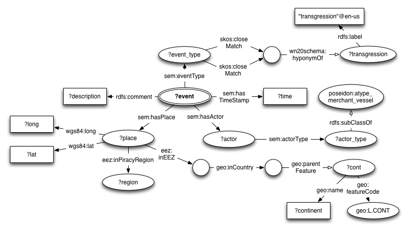
The queries will match parts of this graph.
Let's write a query that gets all piracy events and the geographical region where these events took place. The events are described in the Simple Event Model, where events are linked to the places where they happen. In the case of the Linked Open Piracy data set, these places are categorized in regions with the eez:inPiracyRegion property. To gather all the events and their associated regions, you can use the following query and fire it by calling the SPARQL function. Every variable in the SPARQL query will correspond to a column in a result table data frame.
q <- paste(sparql_prefix,
  "SELECT *
   WHERE {
     ?event sem:hasPlace ?place .
     ?place eez:inPiracyRegion ?region .
   }")

res <- SPARQL(endpoint,q,ns=prefix,extra=options)$results

res
# output:
#                 event                    place                     region
# 1  lop:event_2005_001 lop:place_event_2005_001     eez:Region_Middle_East
# 2  lop:event_2005_002 lop:place_event_2005_002    eez:Region_India_Bengal
# 3  lop:event_2005_003 lop:place_event_2005_003    eez:Region_India_Bengal
# 4  lop:event_2005_004 lop:place_event_2005_004       eez:Region_Indonesia
# 5  lop:event_2005_005 lop:place_event_2005_005       eez:Region_Indonesia
# 6  lop:event_2005_006 lop:place_event_2005_006       eez:Region_Caribbean
# 7  lop:event_2005_007 lop:place_event_2005_007    eez:Region_India_Bengal
# 8  lop:event_2005_008 lop:place_event_2005_008       eez:Region_Indonesia
# 9  lop:event_2005_009 lop:place_event_2005_009 eez:Region_South-East_Asia
# 10 lop:event_2005_010 lop:place_event_2005_010   eez:Region_South_America
# ...
Visualizing counts with a table and pie chart
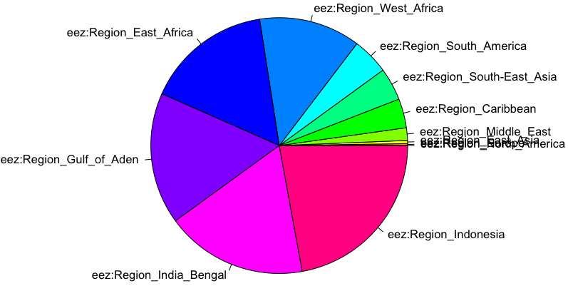
Now that we have some data we can count the number of events per region. This is accomplished with the table function applied to the region column. We can sort the table, and draw a pie chart in rainbow colors like this:
count_per_region <- table(res$region)
sorted_counts <- sort(count_per_region)

sorted_counts
# output:
#   eez:Region_North_America          eez:Region_Europe       eez:Region_East_Asia
#                          1                          4                         11
#     eez:Region_Middle_East       eez:Region_Caribbean eez:Region_South-East_Asia
#                         39                         86                         95
#   eez:Region_South_America     eez:Region_West_Africa     eez:Region_East_Africa
#                        103                        309                        354
#    eez:Region_Gulf_of_Aden    eez:Region_India_Bengal       eez:Region_Indonesia
#                        402                        455                        530
pie(sorted_counts, col=rainbow(12))
This yields the following pie chart:
Visualizing two variables with a two-way table and a stacked barchart
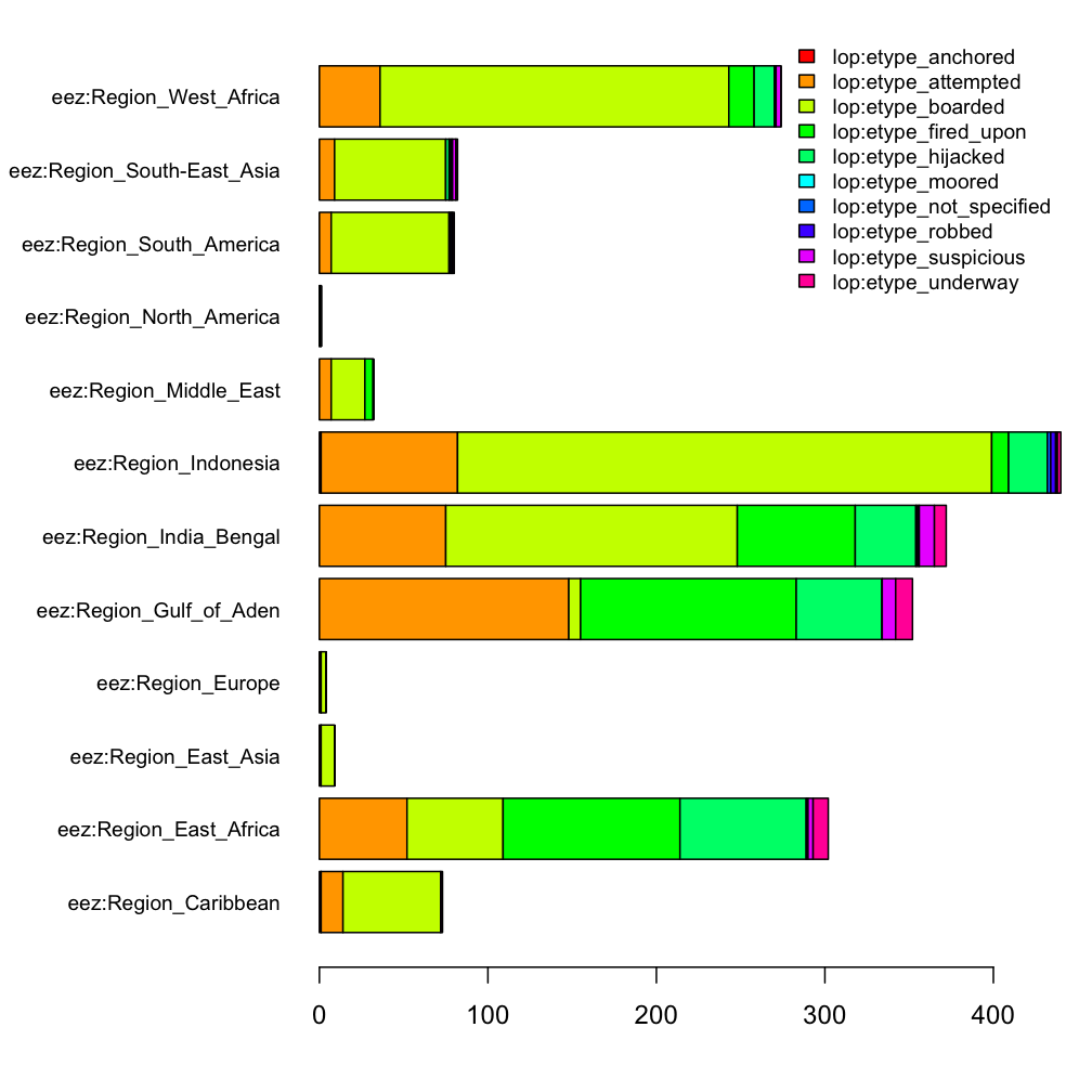
With a little more effort you can plot a which types of events happen per region. To accomplish this we will have to adapt the query to also retrieve the type of event. The updated query looks like this:
q <- paste(sparql_prefix,
  "SELECT *
   WHERE {
     ?event sem:eventType ?event_type .
     ?event sem:hasPlace ?place .
     ?place eez:inPiracyRegion ?region .
   }")
res <- SPARQL(endpoint,q,ns=prefix,extra=options)$results
You can do a conditional count table, in this case event type count per region like this:
event_region_table <- table(res$event_type,res$region)
To plot this table with the appropriate margin and legend you can use the following three lines of code:
par(mar=c(4,10,1,1))
barplot(event_region_table, col=rainbow(10), horiz=TRUE, las=1, cex.names=0.8)
legend("topright", rownames(event_region_table),
       cex=0.8, bty="n", fill=rainbow(10))
This yields the following stacked barchart:
Putting observations on a map
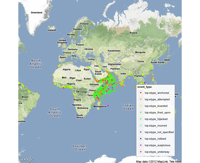
Now, if we want to see where these typed events actually happen in the world, we similarly extend the query to fetch the latitude and longitude of each event and use the ggmap package to plot them on the map with the same colors as before.
q <- paste(sparql_prefix,
  "SELECT *
   WHERE {
     ?event sem:eventType ?event_type .
     ?event sem:hasPlace ?place .
     ?place wgs84:lat ?lat .
     ?place wgs84:long ?long .
   }")
res <- SPARQL(endpoint,q,ns=prefix,extra=options)$results
We use the gmap function to fetch a Google map centered on the Gulf of Aden at zoom level 2. We tell the ggmap package to use the event_type column in the result data frame to determine the color and to the the lat and long columns to set the x and y coordinate on the map. with the geom_point function. The colors are set with the scale_color_manual function.
qmap('Gulf of Aden', zoom=2, legend='bottomright') +
  geom_point(aes(x=long, y=lat, colour=event_type), data=res) +
  scale_color_manual(values = rainbow(10))
With new versions of ggplot2 the legend does not work in the same way. For the sake of simplicity you can leave it away for the moment as follows:
qmap('Gulf of Aden', zoom=2) +
  geom_point(aes(x=long, y=lat, colour=event_type), data=res) +
  scale_color_manual(values = rainbow(10))
This yields the following map:
Filtering literal values
The weaponry used by the pirates is not yet explicitly modeled in RDF in the Linked Open Piracy data set. However, the information IS contained in the textual descriptions of the events which are represented as RDFS comment fields. If we want to show where all the rocket propelled grenade launchers are used (called RPGs in navy lingo, and bazookas by the rest of us) you can narrow down the visualization with a regular expression on the textual description of the event. This can be done as follows:
q <- paste(sparql_prefix,
  "SELECT *
   WHERE {
     ?event rdfs:comment ?description .
     FILTER regex(?description,'RPG','i')
     ?event sem:eventType ?event_type .
     ?event sem:hasPlace ?place .
     ?place wgs84:lat ?lat .
     ?place wgs84:long ?long .
   }")
res <- SPARQL(endpoint,q,ns=prefix,extra=options)$results

qmap('Gulf of Aden', zoom=2, legend='bottomright') +  # or "qmap('Gulf of Aden', zoom=2)" for new ggplot2 versions
  geom_point(aes(x=long, y=lat, colour=event_type), data=res) +
  scale_color_manual(values = rainbow(10))
This yields the following map:
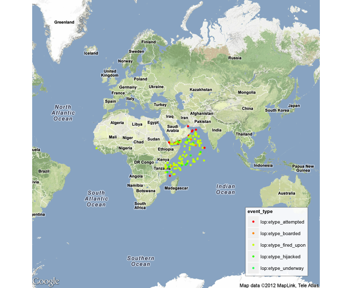
This makes it immediately clear that RPGs are involved mostly in (attempted) hijackings near Somalia. Most of the piracy occurs in Indonesia, but is clearly of an entirely different sort.
Computing correlations
Another thing you can do with the two-way tables you can create with the table function is compute correlations. For example, we could correlate regions in the world with respect to which kind of ships are attacked or what kind of piracy events happen there. The example below shows exactly these two kinds of correlation. First we collect the co-occurences of event types and regions and actor types and regions.
q <- paste(sparql_prefix,
"SELECT ?event_type ?actor_type ?region
   WHERE {
     ?event sem:eventType ?event_type .
     ?event sem:hasPlace ?place .
     ?place eez:inPiracyRegion ?region .
     ?event sem:hasActor ?actor .
     ?actor sem:actorType ?actor_type .
   }")
res <- SPARQL(endpoint,q,ns=prefix,extra=options)$results
et_region <- table(res$event_type,res$region)
at_region <- table(res$actor_type,res$region)
Now we will correlate regions with respect to which event types occur in these regions and show the Pearson correlation of all the regions with the region Gulf of Aden, sorted in decreasing order.
et_cor <- cor(et_region, method='pearson')
sort(et_cor['eez:Region_Gulf_of_Aden',], decreasing=TRUE)
# output:
#    eez:Region_Gulf_of_Aden     eez:Region_East_Africa   eez:Region_North_America
#                1.000000000                0.767785217                0.549721825
#    eez:Region_India_Bengal     eez:Region_Middle_East          eez:Region_Europe
#                0.434693409                0.191477407                0.069687244
#       eez:Region_Indonesia       eez:Region_Caribbean     eez:Region_West_Africa
#                0.028176481                0.004955375               -0.001138778
# eez:Region_South-East_Asia   eez:Region_South_America       eez:Region_East_Asia
#               -0.069604873               -0.098527227               -0.098686326
You can see that there is only one strongly correlated region, which is East Africa (out of the coast of Somalia). The rest is weakly correlated. If we look at the correlation of the regions with respect to the types of ships that are attacked, we see a different picture.
at_cor <- cor(at_region, method='pearson')
sort(at_cor['eez:Region_Gulf_of_Aden',], decreasing=TRUE)
# output:
#    eez:Region_Gulf_of_Aden    eez:Region_India_Bengal       eez:Region_Indonesia
#                 1.00000000                 0.92107990                 0.91819311
#       eez:Region_East_Asia     eez:Region_West_Africa     eez:Region_Middle_East
#                 0.87295516                 0.84970719                 0.81460659
#   eez:Region_South_America       eez:Region_Caribbean     eez:Region_East_Africa
#                 0.69429767                 0.68776759                 0.68691583
# eez:Region_South-East_Asia          eez:Region_Europe   eez:Region_North_America
#                 0.68554899                 0.57979269                 0.01544673
Regions are much more similar with respect to the victim ship types. A region that stands out is Indonesia. Quite similar kinds of ships are attached as in the Gulf of Aden (big ships, although they are not underway but anchored, usually), but what happens to them is completely different (boarding and then theft, not hijacking).
Generalization using rdfs:subClassOf reasoning
Let's say we want to see what kind of attacks happen to merchant ships (e.g. bulk carriers, tankers). What we can do to accomplish this is use RDFS subClassOf reasoning over the actor type to check whether the victim ship type is a kind of merchant vessel.
q <- paste(sparql_prefix,
  "SELECT *
   WHERE {
     ?event sem:eventType ?event_type .
     ?event sem:hasActor ?actor .
     ?actor sem:actorType ?actor_type .
     ?actor_type rdfs:subClassOf poseidon:atype_merchant_vessel .
   }")
res <- SPARQL(endpoint,q,ns=prefix,extra=paste(options,"entailment=rdfs"))$results

mv_et_table <- table(res$event_type)

mv_et_table
# output:
#      lop:etype_anchored     lop:etype_attempted       lop:etype_boarded    lop:etype_fired_upon
#                       2                     474                     997                     383
#      lop:etype_hijacked        lop:etype_moored lop:etype_not_specified        lop:etype_robbed
#                     164                       3                       2                       6
#    lop:etype_suspicious      lop:etype_underway
#                      25                      26
Using a statistical test to compare distributions
If we compare this to the number of events of other vessel types, we can do a chi-square test to see if this distribution is significantly different to the attacks on merchant vessels.
q <- paste(sparql_prefix,
  "SELECT *
   WHERE {
     ?event sem:eventType ?event_type .
     ?event sem:hasActor ?actor .
     ?actor sem:actorType ?actor_type .
   }")
res <- SPARQL(endpoint,q,ns=prefix,extra=options)$results

all_et_table <- table(res$event_type)
Now we deduct the number of events on merchant vessels from the number of events on all vessels to get the number of attacks on non-merchant vessels. Now we can do a chi-square test to test the equivalence of mv_et_table and rest_et_table.
rest_et_table <- all_et_table - mv_et_table

rest_et_table
# output:
#      lop:etype_anchored     lop:etype_attempted       lop:etype_boarded    lop:etype_fired_upon
#                       0                      43                     166                      44
#      lop:etype_hijacked        lop:etype_moored lop:etype_not_specified        lop:etype_robbed
#                      77                       0                       2                       0
#    lop:etype_suspicious      lop:etype_underway
#                       7                       3
chisq.test(mv_et_table,rest_et_table)
# output:
#
# Pearson's Chi-squared test
#
# data:  as.vector(rest) and as.vector(mv)
# X-squared = 63.3333, df = 56, p-value = 0.2336
You can see that the probability of the difference between the two distributions is due to chance is 0.2336. At a confidence level of 0.05 this means we should conclude they are equal.
Wrap-up
In this tutorial we showed how to do simple visualizations of data in the Linked Open Piracy data set using the SPARQL Package for R. We also showed how to compute the Pearson correlation between two multinomial distributions (between two sets of counts of URIs) and how to do a statistical test, the chi-square test to determine whether or not the difference between two such distributions can be attributed to chance or not.

VU University Amsterdam R Tutorials by Willem Robert van Hage is licensed under a Creative Commons Attribution-ShareAlike 3.0 Unported License.
This tutorial has been developed within the COMBINE project supported by the ONR Global NICOP grant N62909-11-1-7060.